How to Read the Bloch Sphere

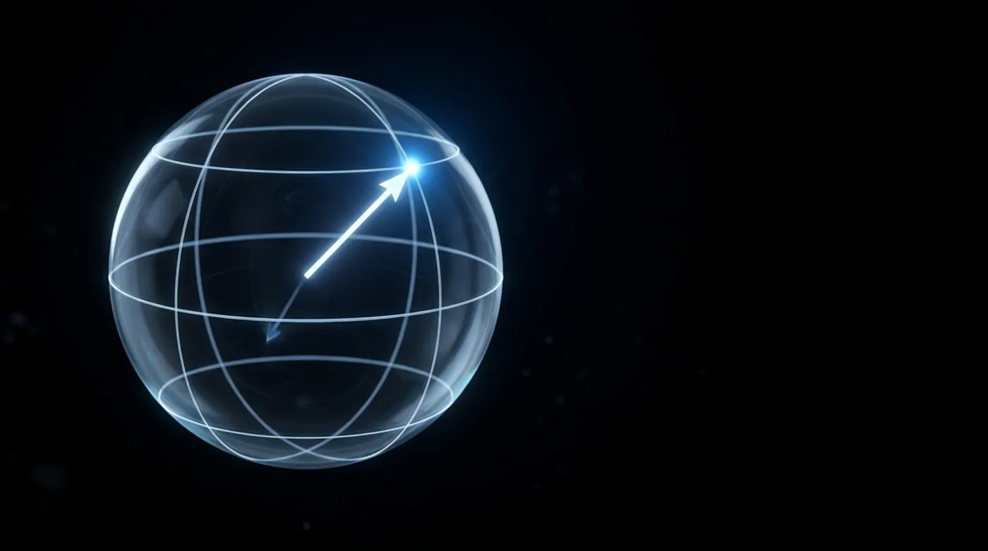
The Bloch sphere is the single most useful picture in quantum computing, and it is also the one most often waved at and never explained. This series fixes that. Over five parts we drive the interactive Bloch sphere simulator on this site, gate by gate, and every screenshot below is a real state the simulator produced. You can reproduce all of them yourself by clicking the same buttons.

This first part covers only one skill: reading the picture. No gates yet. By the end you will be able to look at any arrow on the sphere and say what the qubit is, what a measurement would do to it, and how it differs from the state next to it.

The map before the journey

Here is the sphere with nothing on it but its own geography.

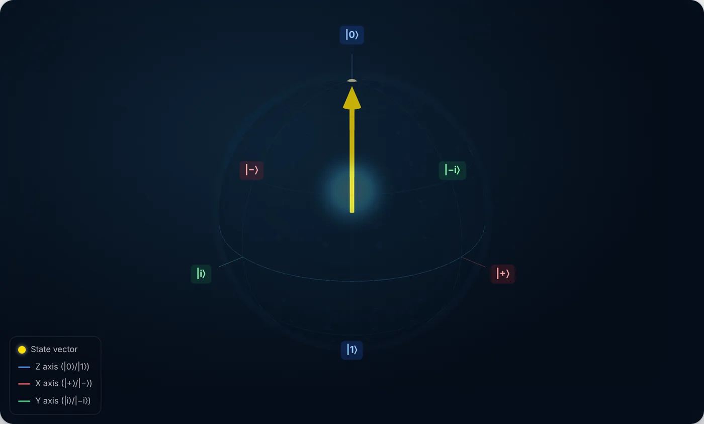
Three things to notice.

Every point on the surface is a legal qubit state. Not just the six labelled ones. The surface is the complete catalogue of everything a single qubit can be. There is nothing else.

The arrow is the qubit. One arrow, one state. It always reaches the surface, never stops short.

The two poles are the classical bits. The north pole is |0⟩, the south pole is |1⟩. If your qubit’s arrow is parked on a pole, it is behaving like an ordinary bit and there is nothing quantum going on.

Everywhere else is superposition.

Latitude is the odds

Start the simulator and it sits at |0⟩, straight up.

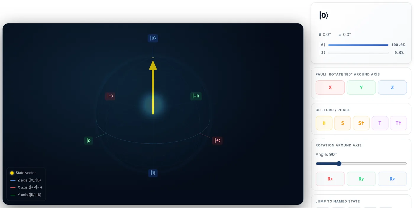
The readout panel gives you two angles and two probabilities. The angle that matters right now is θ (theta), the polar angle measured down from the north pole. At the north pole θ is 0, and the qubit measures as 0 with 100% certainty.

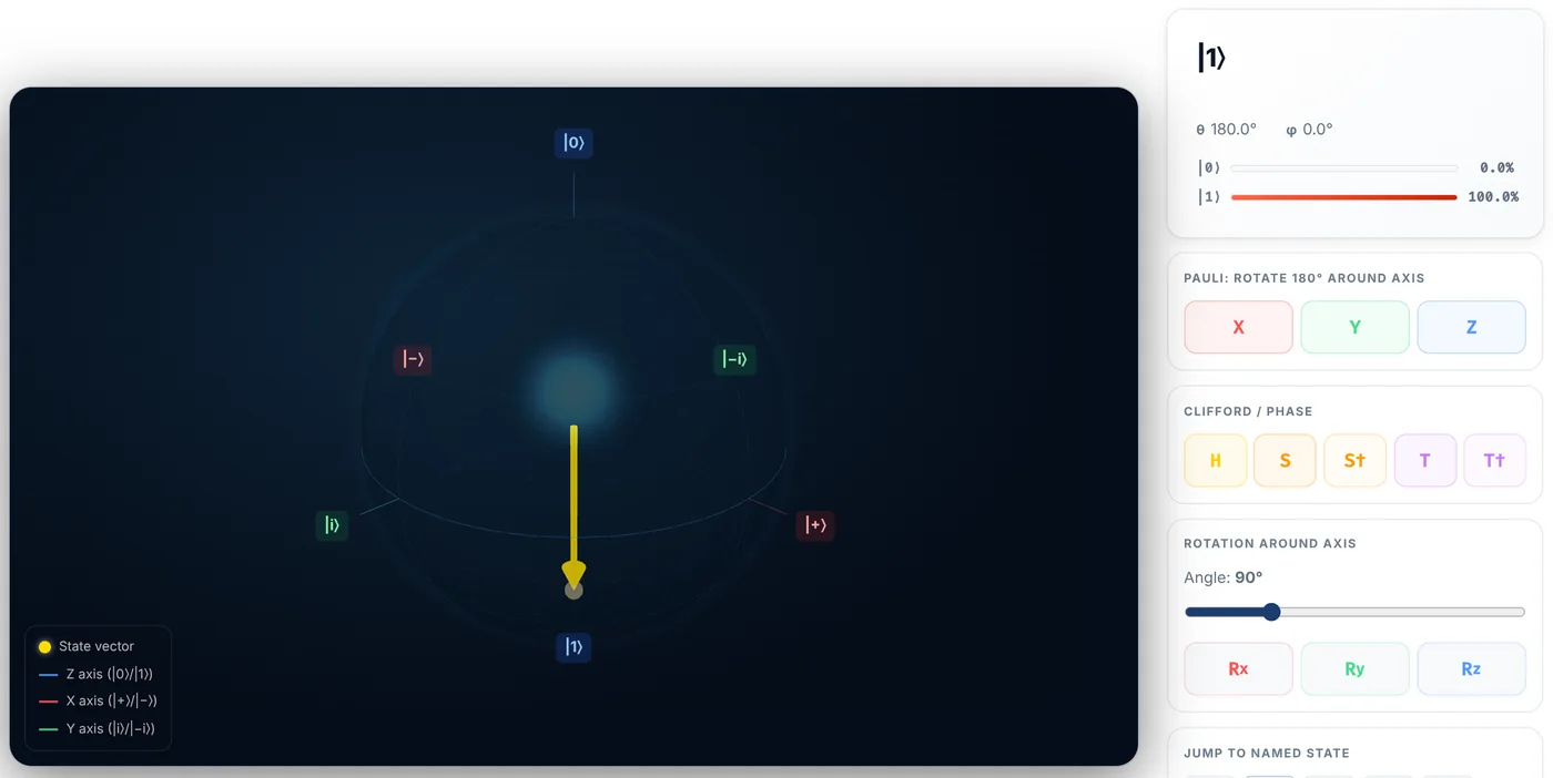
Click the |1⟩ button and the arrow swings to the south pole.

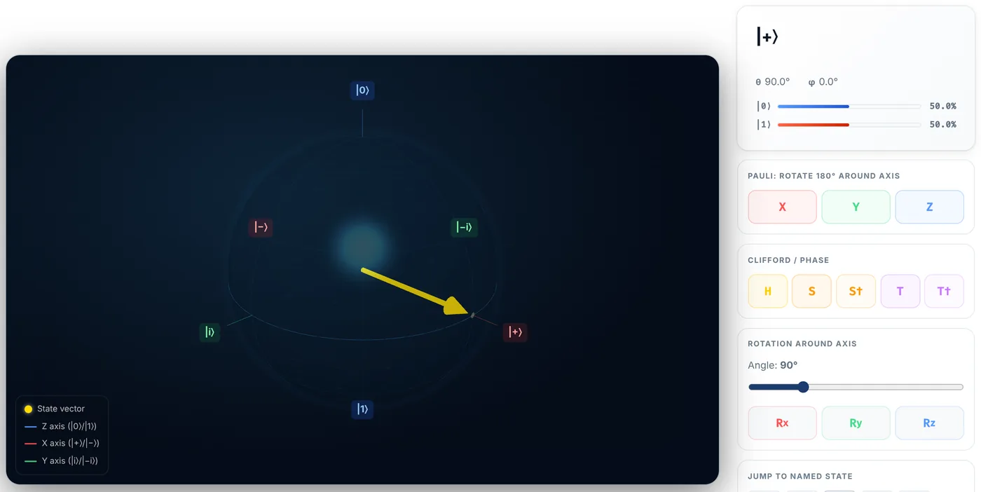
Halfway between them, on the equator, the odds are even. Click |+⟩:

That is the whole rule, and it is worth committing to memory:

Height on the sphere is the measurement probability. How far down the arrow tilts, and nothing else, decides the odds of getting 0 or 1.

The exact relationship is P(0) = cos²(θ/2). Drop the arrow to θ = 60° and you should get cos²(30°) = 0.75, so 75% zeros. The simulator agrees:

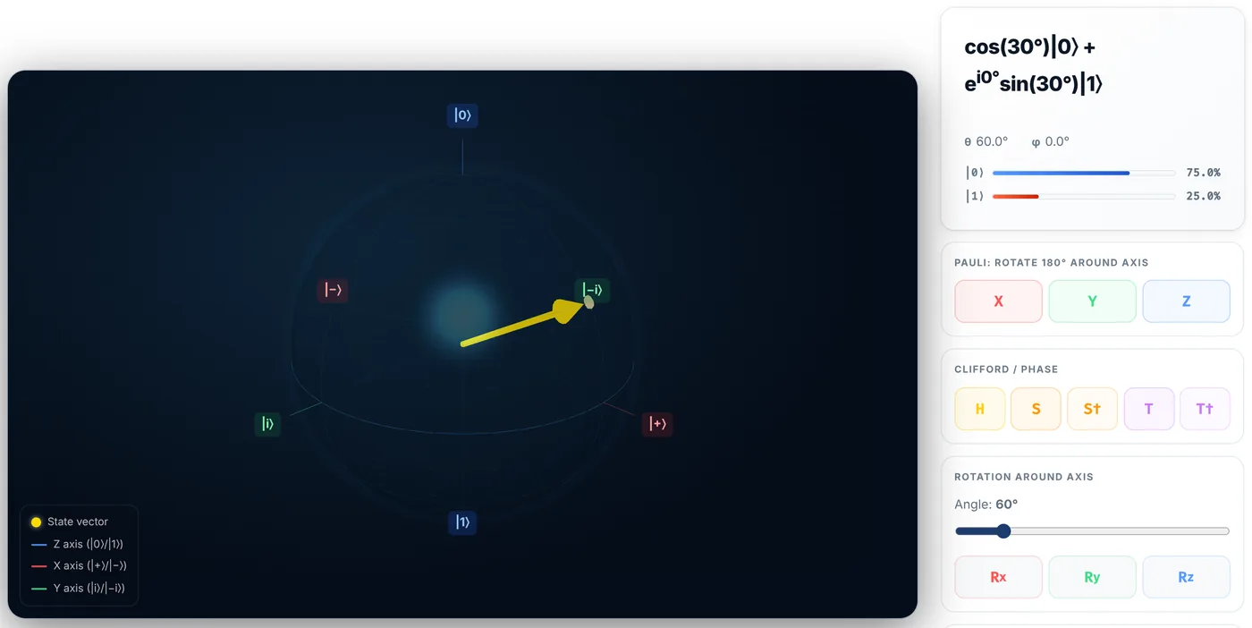
That θ/2 catches people out. A 60° tilt does not mean the state is “60% of the way to |1⟩”. The amplitudes carry cos(θ/2) and sin(θ/2), and the probabilities are their squares. Part 4 comes back to why the half-angle is there.

Longitude is the phase, and it is invisible to a measurement

Now the part that makes the sphere worth drawing. Click |i⟩ and watch the arrow swing around the equator to a different place, staying at the same height.

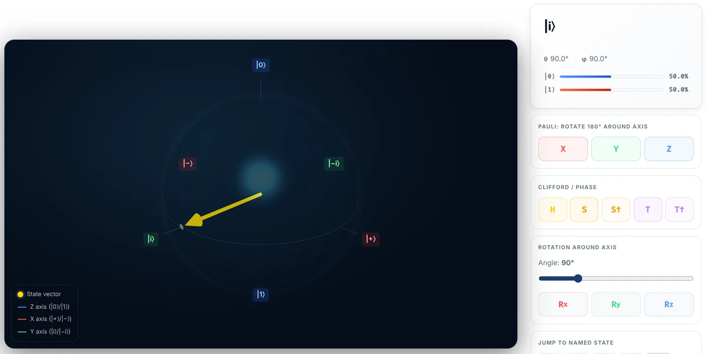
Compare that readout with the |+⟩ one above. The probability bars are identical. Both are 50/50. Yet |+⟩ and |i⟩ are genuinely different states, and a quantum computer can tell them apart perfectly.

The difference lives in φ (phi), the azimuthal angle going around the sphere, and φ is the relative phase. It contributes nothing to the odds of a Z measurement, which is why the bars do not move. What it does control is how the state behaves when you interfere it with something else. Phase is where quantum algorithms actually do their work: Grover’s, Shor’s and the quantum Fourier transform are all machines for pushing φ around until the phases cancel on the wrong answers and reinforce on the right one.

So the second rule:

The angle around the sphere is phase. Measurement in the computational basis cannot see it. Interference can.

Put the two together and the general state is:

|ψ⟩ = cos(θ/2)|0⟩ + e^(iφ) sin(θ/2)|1⟩

θ sets the size of the two amplitudes. φ sets the phase between them. Two angles, two degrees of freedom, one sphere.

Checking the readout in Qiskit

The simulator is not doing anything you cannot reproduce in ten lines. This converts a statevector into the same θ and φ the panel shows.

import numpy as np
from qiskit.quantum_info import Statevector

def bloch_angles(sv):
    """Return (theta, phi) in degrees for a single-qubit statevector."""
    a, b = sv.data                       # amplitudes of |0> and |1>
    if abs(a) > 1e-9:
        # Rotate away the global phase so the |0> amplitude is real and positive.
        b = b * np.exp(-1j * np.angle(a))
        a = abs(a)
    theta = 2 * np.arccos(min(1.0, abs(a)))
    phi = np.angle(b) if abs(b) > 1e-9 else 0.0
    return np.degrees(theta), np.degrees(phi) % 360

named = {
    "|0>": Statevector([1, 0]),
    "|1>": Statevector([0, 1]),
    "|+>": Statevector(np.array([1, 1]) / np.sqrt(2)),
    "|i>": Statevector(np.array([1, 1j]) / np.sqrt(2)),
}

for name, sv in named.items():
    theta, phi = bloch_angles(sv)
    p0, p1 = np.abs(sv.data) ** 2
    print(f"{name:4}  theta={theta:6.1f}  phi={phi:6.1f}   P(0)={p0:.2f}  P(1)={p1:.2f}")

|0>   theta=   0.0  phi=   0.0   P(0)=1.00  P(1)=0.00
|1>   theta= 180.0  phi=   0.0   P(0)=0.00  P(1)=1.00
|+>   theta=  90.0  phi=   0.0   P(0)=0.50  P(1)=0.50
|i>   theta=  90.0  phi=  90.0   P(0)=0.50  P(1)=0.50

There is |+⟩ and |i⟩ again: same probabilities, 90° apart in φ. The numbers match the panel exactly.

And the 60° tilt from the screenshot above:

from qiskit import QuantumCircuit

qc = QuantumCircuit(1)
qc.ry(np.radians(60), 0)          # tilt 60 degrees away from the north pole
sv = Statevector(qc)

theta, phi = bloch_angles(sv)
print(f"theta={theta:.1f}  phi={phi:.1f}  P(0)={abs(sv.data[0]) ** 2:.3f}")
print(f"cos^2(theta/2) = {np.cos(np.radians(theta) / 2) ** 2:.3f}")

theta=60.0  phi=0.0  P(0)=0.750
cos^2(theta/2) = 0.750

The one thing beginners get backwards

Two states are perfectly distinguishable (orthogonal) when their arrows point in opposite directions, not when they are at right angles. |0⟩ and |1⟩ are opposite poles. |+⟩ and |−⟩ are opposite ends of the X axis.

Arrows at 90° on the sphere are not orthogonal states. The overlap between two states whose Bloch vectors are γ apart is:

|⟨ψ₁|ψ₂⟩|² = cos²(γ/2)

For γ = 90° that gives 0.5, so |0⟩ and |+⟩ have a 50% overlap and one measurement cannot separate them reliably. Even the single best measurement allowed by physics still guesses wrong about 15% of the time. Only at γ = 180° does the overlap fall to zero and the two states become perfectly distinguishable.

This is the same factor of two showing up again. Angles on the Bloch sphere are always double the angles in the underlying state space. It is the price of squashing a complex two-dimensional space down to a picture you can hold in your hand.

What you can now read

Given any arrow on the sphere, you can state:

• How far down it points (θ) gives you the measurement odds: P(0) = cos²(θ/2).
• Which way round it points (φ) gives you the relative phase, which no computational-basis measurement will ever reveal.
• Opposite arrows are perfectly distinguishable states. Everything else overlaps.
• The surface is the whole story for a single isolated qubit. Nothing lives inside the ball, yet. Part 5 explains what changes when it does.

Open the simulator and click through the six named states until the readout stops surprising you. Then carry on to Part 2, where the arrow finally starts to move and every quantum gate turns out to be nothing more exotic than a rotation.