Measurement, Decoherence and What the Bloch Sphere Cannot Show You

Four parts in, the simulator has given you complete control of a qubit. You can put the arrow anywhere and you know which rotation puts it there.

This part is about the three things the picture will not tell you. Every one of them is the point at which a working intuition either survives contact with real hardware or falls over.

Measurement: the arrow snaps to a pole

Everything so far has been reversible. Every gate was a rotation, and every rotation can be undone by turning back.

Measurement is not a rotation, and it cannot be undone.

Prepare a state with a 60° tilt and look at the readout:

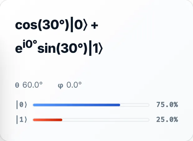
Measure this qubit in the computational basis and two things happen at once. You get one classical bit, 0 with probability 75% and 1 with probability 25%, following the Born rule. And the state jumps to whichever pole matched the outcome. The arrow does not tilt back gracefully. It snaps to |0⟩ or to |1⟩, and everything else about it, the exact latitude, the entire longitude, is gone.

Three consequences that trip people up constantly:

One shot tells you almost nothing. A single measurement of the state above returns “0”. So would a measurement of |0⟩ itself. One bit out of a two-real-parameter state is a terrible exchange rate, which is why quantum algorithms are judged by how well they concentrate the right answer into the probabilities before anyone measures.

You cannot read the arrow. There is no operation that hands you θ and φ. To find out where the arrow was, you must prepare the same state many times over and measure it repeatedly, and even then you only recover the statistics. That process is quantum state tomography, and the Bloch coordinates are exactly what it reconstructs, because the three components of the Bloch vector are the three Pauli expectation values:

x = ⟨X⟩     y = ⟨Y⟩     z = ⟨Z⟩

Measuring “in a different basis” means rotating first. The hardware can only ever read the Z axis, the poles. If you want to measure along X instead, you cannot turn the detector, so you turn the qubit: apply H to bring the X axis into the Z position, then measure. Part 3 showed H doing precisely that swap. Every “measure in the X basis” instruction in every textbook is that trick.

Notice what the simulator never offers you: a Measure button. That is honest. It models pure states evolving unitarily, and measurement is where that model ends.

The circuit is a list of rotations

The panel keeps a running list of what you have applied.

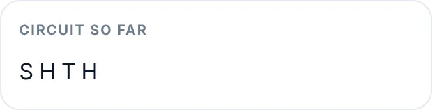
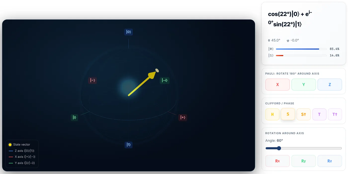
That last observation is the whole of the rest of this article. The arrow never leaves the surface. No sequence of buttons will shorten it. That is not a limitation of the simulator’s code, it is a true statement about unitary evolution of an isolated qubit: rotations preserve length, so a state that starts pure stays pure forever.

Real qubits are not isolated, and real qubits do not stay pure.

Inside the ball: decoherence

A qubit that has interacted with its environment is no longer described by a point on the surface. It is described by a density matrix, and its Bloch vector is shorter than 1. It lives inside the ball.

The length of the vector is a purity meter:

• Length 1, on the surface: a pure state. Everything in Parts 1 to 4.
• Length between 0 and 1: a mixed state. The qubit is partly randomised.
• Length 0, dead centre: the maximally mixed state. A coin flip in every basis, carrying no quantum information whatsoever.

Decoherence is the arrow sinking toward the middle, and the two standard timescales are two different ways of sinking. T1, energy relaxation, drags the vector toward the north pole as the qubit dumps energy and decays to |0⟩. T2, dephasing, kills the x and y components while leaving z alone: the arrow collapses onto the vertical axis, which destroys the phase and therefore destroys interference, while leaving the measurement probabilities untouched.

That second one deserves a moment. Dephasing takes |+⟩, a perfectly good state with a definite phase, and turns it into a 50/50 classical mixture of |0⟩ and |1⟩. The probability bars look identical before and after. Nothing you can see in the Z measurement statistics has changed. But the qubit has stopped being quantum, and any algorithm relying on interference is now returning noise. This is why coherence time, not qubit count, is the number to watch.

You can watch the vector shrink in Qiskit. Depolarising noise mixes the state with the maximally mixed state, and the Bloch vector scales down by exactly the noise parameter:

import numpy as np
from qiskit.quantum_info import Statevector, DensityMatrix, Pauli

def bloch_vector(state):
    """The Bloch vector IS the triple of Pauli expectation values."""
    return [round(float(state.expectation_value(Pauli(p)).real), 3) for p in ("X", "Y", "Z")]

plus = DensityMatrix(Statevector(np.array([1, 1]) / np.sqrt(2)))
maximally_mixed = np.eye(2) / 2

for p in (1.0, 0.6, 0.0):
    rho = DensityMatrix(p * plus.data + (1 - p) * maximally_mixed)
    v = bloch_vector(rho)
    print(f"p={p:.1f}  bloch={v}  length={np.linalg.norm(v):.2f}  purity={float(rho.purity().real):.3f}")

p=1.0  bloch=[1.0, 0.0, 0.0]  length=1.00  purity=1.000
p=0.6  bloch=[0.6, 0.0, 0.0]  length=0.60  purity=0.680
p=0.0  bloch=[0.0, 0.0, 0.0]  length=0.00  purity=0.500

At p = 1 the state is |+⟩ on the surface. At p = 0 the arrow has vanished into the centre and the qubit is worthless. Purity slides from 1 down to 0.5, its minimum for a single qubit.

Nothing in the simulator can produce those middle rows, because it has no noise model. Keep that asterisk attached to every intuition you take from it.

No arrow at all: entanglement

The second edge of the map is harder, and more important.

Two qubits are not two Bloch spheres. A two-qubit pure state needs six real parameters, not four, and once you allow mixed states it takes fifteen. There is no three-dimensional picture of it. The Bloch sphere is a single-qubit tool and it does not generalise.

Worse, the natural fix does not work. If you have an entangled pair and you ask “but what is qubit 0 doing?”, the honest answer is: nothing that a Bloch vector can express. Take a Bell state, trace out the partner qubit, and look at what is left:

from qiskit import QuantumCircuit
from qiskit.quantum_info import partial_trace

bell = QuantumCircuit(2)
bell.h(0)
bell.cx(0, 1)
bell_state = Statevector(bell)

for q in (0, 1):
    reduced = partial_trace(bell_state, [1 - q])
    print(f"qubit {q}:  bloch={bloch_vector(reduced)}  purity={float(reduced.purity().real):.2f}")

qubit 0:  bloch=[0.0, 0.0, 0.0]  purity=0.50
qubit 1:  bloch=[0.0, 0.0, 0.0]  purity=0.50

Both qubits are at the origin. Both are maximally mixed. Individually they are worthless, indistinguishable from a qubit that has fully decohered, and yet together they are the most strongly correlated state two qubits can be in.

Qiskit’s own Bloch plotter, asked to draw a Bell state, produces this:

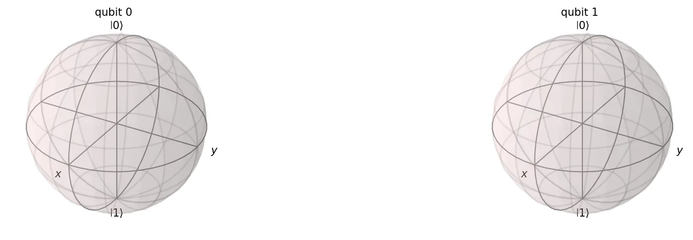
Two empty spheres. Every scrap of information in a Bell state lives in the correlation between the qubits, and correlation is precisely what a per-qubit picture throws away. This is the deepest limitation of the Bloch sphere and the reason it stops being useful the moment your circuit gets interesting: entanglement, the resource that makes quantum computing worth doing, is invisible to it.

The map and its edges

The Bloch sphere earns its place. For a single isolated qubit it is exact, complete, and it turns gate algebra into geometry you can see. Almost everything in Parts 1 to 4 is easier to see than to prove.

Just carry the three asterisks with you:

The picture says	The truth is
The arrow always has length 1	Real qubits decohere and sink inside the ball
Every state is a point on a sphere	Only for one qubit, and only when it is unentangled
Gates rotate the arrow	Measurement does not rotate it, it destroys it

A map with known edges is a good map. A map you have mistaken for the territory is how people end up believing a qubit is “both 0 and 1 at the same time”, which is a sentence the sphere never says.

Where to go next

You have the geometry. The natural next steps:

• The mathematics behind the sphere, if you want the SU(2) and SO(3) machinery underneath, plus tomography and gate approximation in full.
• Build your first quantum circuit in Qiskit, to put two qubits together and meet the entanglement this picture cannot draw.
• The circuit builder, where you can drop an H and a CNOT onto two qubits and read the Bell state off the amplitudes and probability bars directly. It deliberately shows no Bloch spheres, and this article is the reason it cannot.

And the simulator is always there. Most of what you now know came out of clicking its buttons and paying attention.