Getting Started with Qiskit

If you already know Python and want to start writing quantum programs, Qiskit is the strongest place to begin. It is IBM’s open-source quantum computing SDK, and it has the largest community of any quantum programming framework: over 600 contributors on GitHub, extensive documentation, and a free tier that gives you access to real quantum hardware (not just simulators). Other frameworks like Cirq and PennyLane are excellent for specific use cases, but Qiskit offers the broadest path from “first circuit” to “running on real processors” with the least friction. If you can write a Python function, you can write a quantum circuit.

This tutorial walks you through installing Qiskit, building and running your first quantum circuit, and understanding every line of what you wrote. By the end, you will have run a real quantum computation and understood the physics behind the result.

Prerequisites

You need Python 3.9 or newer and pip. No quantum physics background is required. If you are comfortable writing for loops and calling functions in Python, you have everything you need.

Installing Qiskit

Qiskit is distributed as a standard Python package. The core qiskit package contains the circuit-building tools and transpiler. The qiskit-ibm-runtime package provides the client for sending circuits to IBM’s cloud quantum hardware. The qiskit-aer package gives you a high-performance local simulator for testing before you use real hardware. Install all three:

pip install qiskit qiskit-ibm-runtime qiskit-aer

To confirm everything installed correctly, run the following. This just imports Qiskit and prints its version number:

import qiskit
print(qiskit.__version__)  # Output: 2.3.1

If you see a version number starting with 2, you are ready to go. If you get an import error, double-check that you installed into the correct Python environment (virtual environments are strongly recommended).

Your first quantum circuit: the Bell state

Classical bits are either 0 or 1. Qubits can be in a superposition of both, and multiple qubits can be entangled so that measuring one instantly determines the other. The simplest circuit that demonstrates both of these properties is called a Bell state, and it is the “Hello World” of quantum computing.

Here is the plan in plain English: take two qubits that both start as 0, put the first one into superposition (so it is equally likely to be 0 or 1), then entangle it with the second qubit, and finally measure both. The result will show something impossible in classical computing: two bits that are perfectly correlated without any classical communication between them.

The following code creates a quantum circuit with two qubits (the quantum register) and two classical bits (where the measurement results will be stored). It applies two gates and then measures:

from qiskit import QuantumCircuit

# Create a circuit with 2 qubits and 2 classical bits
qc = QuantumCircuit(2, 2)

# Put qubit 0 into superposition
qc.h(0)

# Entangle qubit 0 with qubit 1
qc.cx(0, 1)

# Measure both qubits
qc.measure([0, 1], [0, 1])

# Draw the circuit
print(qc.draw())

Output:

     ┌───┐     ┌─┐   
q_0: ┤ H ├──■──┤M├───
     └───┘┌─┴─┐└╥┘┌─┐
q_1: ─────┤ X ├─╫─┤M├
          └───┘ ║ └╥┘
c: 2/═════════════╩══╩═
                0  1 

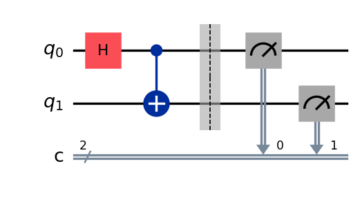
Reading the circuit left to right: qubit 0 passes through the H gate (the box labeled “H”), then a line connects it to the X gate on qubit 1 (this is the CNOT gate, drawn as a vertical connection with a dot on the control qubit and a plus on the target). Finally, both qubits are measured (the “M” boxes), and results flow down into the classical register c.

What just happened?

Let’s break down each operation and the physics behind it.

The Hadamard gate (qc.h(0)) takes qubit 0 from its starting state of |0> and puts it into an equal superposition of |0> and |1>. Think of it this way: before the gate, if you measured qubit 0, you would always get 0. After the gate, you would get 0 half the time and 1 half the time, with genuine quantum randomness (not pseudorandom, truly unpredictable). At this point, qubit 1 is still definitely |0>.

The CNOT gate (qc.cx(0, 1)) is a two-qubit gate that creates entanglement. “CNOT” stands for Controlled-NOT: it flips the target qubit (qubit 1) if and only if the control qubit (qubit 0) is |1>. Since qubit 0 is in superposition, something remarkable happens. The CNOT does not simply flip or not flip qubit 1. Instead, it creates a combined quantum state where both qubits are correlated: when qubit 0 is |0>, qubit 1 stays |0>, and when qubit 0 is |1>, qubit 1 becomes |1>. The two qubits are now entangled, meaning their fates are linked in a way that has no classical equivalent.

The measurement (qc.measure(...)) collapses the quantum state into definite classical values. Before measurement, the two qubits exist in a superposition of |00> and |11> simultaneously. The act of measuring forces the system to “choose” one outcome. Crucially, because the qubits are entangled, they always choose together: you will never see one qubit give 0 while the other gives 1.

Running on a simulator

Before using real quantum hardware (which has limited availability and queue times), you should test your circuits locally using a simulator. The AerSimulator runs on your laptop and behaves like a perfect, noise-free quantum computer.

The following code executes the Bell state circuit 1,024 times (called “shots”) and counts how often each outcome occurs:

from qiskit_aer import AerSimulator

sim = AerSimulator()
result = sim.run(qc, shots=1024).result()
counts = result.get_counts()
print(counts)
# Output: {'00': ~512, '11': ~512}  (roughly 50/50 between 00 and 11)

Understanding the results

The output {'00': ~512, '11': ~512} means that out of 1,024 shots, roughly half produced the outcome 00 (both qubits measured as 0) and the other half produced 11 (both qubits measured as 1). The split will not be exactly 512/512 each time because each shot is a genuinely random event, just like flipping a fair coin 1,024 times will not give you exactly 512 heads.

The critical observation: you never see 01 or 10 in the results. This is entanglement in action. The two qubits are correlated with 100% reliability. If qubit 0 comes out as 0, qubit 1 is guaranteed to also be 0. If qubit 0 comes out as 1, qubit 1 is guaranteed to be 1. This correlation holds no matter what, and it is the foundation that quantum algorithms exploit to outperform classical ones.

Compare this to classical computing: if you just randomly set two independent bits, you would see all four outcomes (00, 01, 10, 11) with roughly equal probability. The absence of 01 and 10 is the signature of quantum entanglement, and it is something no classical random process can replicate while also being truly random at the individual qubit level.

Running on real IBM quantum hardware

Simulators are useful for testing, but the whole point of Qiskit is access to real quantum processors. IBM offers free access to quantum hardware through the IBM Quantum Platform.

First, sign up for a free account at quantum.ibm.com. After registering, retrieve your API token from your account settings page.

The following code saves your credentials (you only need to do this once), selects the least busy available quantum processor, and submits your circuit using the Sampler primitive. The Sampler is Qiskit Runtime’s interface for running circuits and getting measurement results:

from qiskit_ibm_runtime import QiskitRuntimeService, SamplerV2 as Sampler

# Save your credentials once
QiskitRuntimeService.save_account(channel="ibm_quantum", token="YOUR_API_TOKEN")

# Load and pick a real backend
service = QiskitRuntimeService()
backend = service.least_busy(operational=True, simulator=False)
print(f"Running on: {backend.name}")

# Run with the Sampler primitive
sampler = Sampler(backend)
job = sampler.run([qc])
result = job.result()
print(result[0].data.c.get_counts())

When you run on real hardware, you will notice the results are not as clean as the simulator output. You might see something like {'00': 480, '11': 470, '01': 40, '10': 34}. Those small counts for 01 and 10 are not a bug in your code. They are noise: real quantum processors are imperfect, and qubits can lose their quantum state (decohere) or have gates that are slightly inaccurate. Reducing this noise is one of the biggest active areas of quantum computing research.

Key Qiskit objects to know

As you continue building circuits, you will interact with a small set of core objects repeatedly. Here is what each one does:

• QuantumCircuit: The central object in Qiskit. It defines the sequence of quantum gates and measurements that make up your program. You build your circuit by calling methods on this object.
• qc.h(qubit): Applies the Hadamard gate, which creates an equal superposition of |0> and |1>. This is the most common way to introduce randomness and parallelism into a quantum circuit.
• qc.cx(control, target): Applies the CNOT (Controlled-NOT) gate. It flips the target qubit when the control qubit is |1>. This is the standard way to create entanglement between two qubits.
• qc.measure(qubits, classical_bits): Measures the specified qubits and stores the results in classical bits. Measurement is irreversible: once you measure, the superposition is gone.
• AerSimulator: A high-performance local simulator from the qiskit-aer package. Use it for development and testing. It can simulate ideal (noise-free) circuits and also noisy circuits that mimic real hardware.
• SamplerV2: The Qiskit Runtime primitive for executing circuits on IBM hardware (or cloud simulators). It handles transpilation, optimization, and job management behind the scenes.
• QiskitRuntimeService: The client that connects to IBM’s cloud platform. Use it to list available backends, check queue lengths, and manage your jobs.

Common mistakes

When starting out with Qiskit, these are the errors that trip up almost everyone. Knowing them upfront will save you hours of debugging.

Qubit ordering confusion. Qiskit uses little-endian ordering, which means qubit 0 is the rightmost bit in the output string. So if you see the result '10' from a two-qubit circuit, that means qubit 0 measured as 0 and qubit 1 measured as 1. This is the opposite of what most people expect, and it is the single most common source of confusion for new Qiskit users. When in doubt, label your qubits explicitly and verify with a simple test circuit.

Forgetting to transpile for hardware. Your circuit uses abstract gates, but real quantum processors only support a limited set of native gates (typically CNOT, sqrt(X), Rz, and X). Before running on hardware, your circuit must be transpiled: converted into equivalent operations using only the native gate set and respecting the processor’s qubit connectivity. The SamplerV2 primitive handles this automatically, but if you are running circuits manually through a backend, you need to call transpile() yourself or your job will fail.

Confusing shots with accuracy. Increasing the number of shots (say, from 1,024 to 100,000) gives you a more precise estimate of the probability distribution, but it does not make your quantum circuit more accurate or reduce hardware noise. Each individual shot still runs on the same noisy hardware. More shots means the histogram converges closer to the true probability distribution, like flipping a coin more times gives a ratio closer to 50/50. But if the coin is biased (the hardware is noisy), more flips just reveal the bias more clearly.

Measuring in the wrong basis. The measure() function measures in the computational basis (|0> and |1>) by default. If your algorithm requires measuring in a different basis (such as the X-basis or Y-basis), you need to apply additional gates before measurement. For example, to measure in the X-basis, apply a Hadamard gate before measuring. This is a subtle point that becomes important once you move beyond introductory circuits.

Next steps

Now that you have built and run your first quantum circuit, here is a concrete learning path:

1. Understand the gates. The Hadamard and CNOT gates used in this tutorial are just two of many quantum gates. Learn what the X, Y, Z, S, T, and rotation gates do, and how to think about them as matrix operations. Start with our guide: Quantum Gates Explained.

2. Learn your first quantum algorithm. Grover’s search algorithm is the most intuitive quantum algorithm and a great next step after Bell states. It demonstrates a real quantum speedup on a practical problem (searching an unsorted database). Walk through it step by step: Grover’s Algorithm Explained.

3. Understand entanglement more deeply. The Bell state you built is the simplest example of entanglement, but the concept goes much further. Learn about Bell inequalities, the different Bell states, and why entanglement matters for quantum communication and quantum algorithms: Quantum Entanglement Explained.

4. Master transpilation. When you move from simulators to real hardware, understanding how Qiskit transpiles your circuits is essential for getting good results. Learn about optimization levels, routing, and gate decomposition: Qiskit Transpilation.

5. Explore IBM’s learning resources. IBM maintains a comprehensive learning platform at quantum.cloud.ibm.com/learning with interactive textbooks, video courses, and coding challenges that go well beyond what any single tutorial can cover.