Getting Started with Cirq

Cirq is Google’s open-source Python framework for writing, simulating, and running quantum circuits. It was built by Google’s Quantum AI team and is the same framework they used for their landmark quantum supremacy experiment on the Sycamore processor. The key insight behind Cirq’s design is that qubits are not abstract. Unlike Qiskit, where you create numbered qubits and let the transpiler figure out how to map them onto hardware, Cirq asks you to place qubits on a grid that mirrors the physical layout of a real superconducting chip. This matters because real quantum processors have limited connectivity: a qubit at position (3, 2) can only interact directly with its immediate neighbors, and any two-qubit gate between non-adjacent qubits requires expensive SWAP operations that add noise. By making qubit placement explicit from the start, Cirq encourages you to think about hardware constraints while you design your algorithm, not as an afterthought.

Installation

Install Cirq from PyPI. The base cirq package includes the simulator, core gate library, and all the tools you need for local development.

pip install cirq

Verify that the installation succeeded by printing the version:

import cirq
print(cirq.__version__)

If you plan to run circuits on Google hardware, you will also need the cirq-google package, but for this tutorial the base installation is sufficient.

Core Concept: Qubit Placement

The biggest difference between Cirq and other frameworks is how you define qubits. In Cirq, qubits carry positional information that corresponds to physical hardware. The GridQubit class models the 2D grid layout of superconducting processors like Sycamore, where each qubit sits at a specific row and column.

import cirq

# Grid qubits - match the layout of real superconducting processors
q0 = cirq.GridQubit(0, 0)
q1 = cirq.GridQubit(0, 1)

print(q0)  # q(0, 0)

When you are prototyping an algorithm and do not need to think about physical layout yet, Cirq also provides LineQubit, which arranges qubits in a simple linear chain. This is convenient for textbook circuits where topology is not the focus.

q0, q1, q2 = cirq.LineQubit.range(3)

You can freely mix qubit types across different circuits, but within a single circuit you should stick to one type. When you are ready to run on real hardware, you will switch from LineQubit to GridQubit and map your algorithm onto the processor’s actual connectivity graph.

Building a Bell State Circuit

A Bell state is the simplest demonstration of quantum entanglement: two qubits placed into a superposition where their measurement outcomes are perfectly correlated. Let’s build one step by step. First, the Hadamard gate puts qubit 0 into an equal superposition of |0> and |1>. Then the CNOT gate entangles the two qubits so that qubit 1 always matches qubit 0. Finally, we measure both qubits and label the measurement 'result' so we can retrieve it later.

import cirq

q0, q1 = cirq.LineQubit.range(2)

circuit = cirq.Circuit([
    cirq.H(q0),           # Hadamard on q0
    cirq.CNOT(q0, q1),    # Entangle
    cirq.measure(q0, q1, key='result'),  # Measure both
])

print(circuit)

Output:

0: ───H───@───M('result')───
          │   │
1: ───────X───M─────────────

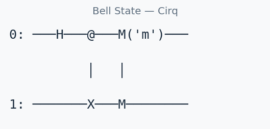
Reading the Circuit Diagram

Cirq’s text-based circuit diagrams are one of its most useful features. Here is what each part means:

• 0: and 1: on the left are qubit labels. Each horizontal line represents one qubit’s timeline, flowing left to right.
• ───H─── is a Hadamard gate acting on qubit 0. The dashes on either side are just wires showing the passage of time.
• @ and X connected by │ represent a CNOT gate. The @ is the control qubit (q0), the X is the target qubit (q1), and the vertical bar shows they are linked. This is standard notation: if the control qubit is |1>, the target qubit gets flipped.
• M('result') is the measurement operation. Both qubits feed into the same measurement gate, grouped under the key 'result'. The │ connecting the two M symbols shows they belong to the same measurement.

Each column of gates in the diagram corresponds to one Moment in Cirq’s internal representation. In this circuit there are three moments: the H gate, the CNOT gate, and the measurement.

Understanding Moments

Cirq organizes every circuit into a sequence of Moments. A Moment is a single time step in which one or more gates execute in parallel, provided they act on different qubits. This is not just a visual convenience; it directly reflects how gates run on real hardware.

Why does parallelism matter? On a real quantum processor, qubits lose their quantum state over time through a process called decoherence. Every microsecond your circuit takes to execute is another microsecond of accumulated noise. A circuit with 10 sequential moments will generally produce better results than an equivalent circuit with 20 moments, even if they apply the same total number of gates. Shorter circuits mean less time for errors to creep in.

Cirq automatically packs independent gates into the same moment when you pass a flat list of operations to cirq.Circuit. In the following example, the two Hadamard gates act on different qubits, so Cirq places them in a single moment:

# Cirq automatically packs independent gates into the same moment
circuit = cirq.Circuit([
    cirq.H(q0),
    cirq.H(q1),     # This runs in the same moment as H(q0) - parallel
    cirq.CNOT(q0, q1),
])

print(circuit)
# 0: ───H───@───
#           │
# 1: ───H───X───

Notice that the diagram shows only two columns: one for both H gates (running simultaneously) and one for the CNOT. If you need explicit control over moment boundaries, you can construct moments manually using cirq.Moment:

circuit = cirq.Circuit([
    cirq.Moment(cirq.H(q0)),        # Moment 0: only H on q0
    cirq.Moment(cirq.H(q1)),        # Moment 1: only H on q1 (sequential, not parallel)
    cirq.Moment(cirq.CNOT(q0, q1)), # Moment 2: CNOT
])

This version has three moments instead of two. On real hardware, it would take longer to execute and accumulate more noise. Explicit moment control is useful when you need to insert barriers or enforce a specific gate ordering for calibration purposes, but in most cases you should let Cirq’s automatic packing do its job.

Simulating Your Circuit

Cirq’s built-in simulator gives you two distinct ways to execute a circuit, and understanding the difference is important for choosing the right one.

run(): Sampling Measurement Outcomes

The run() method treats your circuit the way real hardware would: it executes the circuit many times (controlled by the repetitions parameter) and returns the measurement results as classical bit strings. You never see the underlying quantum state, just the outcomes you would get from repeated experiments.

import cirq

q0, q1 = cirq.LineQubit.range(2)
circuit = cirq.Circuit([
    cirq.H(q0),
    cirq.CNOT(q0, q1),
    cirq.measure(q0, q1, key='m'),
])

simulator = cirq.Simulator()
result = simulator.run(circuit, repetitions=1000)
print(result.histogram(key='m'))
# Counter({0: ~500, 3: ~500})  ← 0=|00⟩, 3=|11⟩

The histogram maps integer values to counts. The integer is the binary measurement result read as a number: 00 in binary is 0, and 11 in binary is 3. You should see roughly equal counts for both, confirming the Bell state produces perfectly correlated outcomes. Use run() when you want to benchmark algorithm success rates, estimate expectation values from samples, or validate circuits that include measurements.

simulate(): Full Statevector Access

The simulate() method computes the exact quantum state of the system after all gates have been applied. This is something no real quantum computer can do (you cannot observe a quantum state without collapsing it), but it is invaluable for debugging and verifying that your circuit produces the correct state.

circuit_no_measure = cirq.Circuit([cirq.H(q0), cirq.CNOT(q0, q1)])
result = simulator.simulate(circuit_no_measure)
print(result.final_state_vector)
# [0.707+0j, 0+0j, 0+0j, 0.707+0j]  ← Bell state |Φ+⟩

The output is a complex-valued vector with one entry per computational basis state. For two qubits, there are four entries corresponding to |00>, |01>, |10>, and |11>. The Bell state has amplitude 0.707 (which is 1/sqrt(2)) on |00> and |11>, and zero on the other two states. Use simulate() when you need to verify amplitudes, debug phase errors in your circuit, or compute quantities like fidelity and entanglement entropy that require the full state description. Note that statevector simulation scales exponentially: it is practical up to about 25-30 qubits on a typical laptop, while run() can sometimes handle slightly larger circuits since it only needs to sample, not store, the full state.

Common Patterns: Inspecting Circuit Structure

As your circuits grow more complex, you will want to inspect their moment structure programmatically rather than just reading diagrams. Cirq makes the internal organization fully accessible through Python.

import cirq

q0, q1, q2 = cirq.LineQubit.range(3)

circuit = cirq.Circuit([
    cirq.H(q0),
    cirq.H(q1),
    cirq.CNOT(q0, q1),
    cirq.H(q2),
    cirq.measure(q0, q1, q2, key='out'),
])

# Print the total number of moments (circuit depth)
print(f"Circuit depth: {len(circuit)} moments")

# Iterate over each moment and list its operations
for i, moment in enumerate(circuit):
    ops = [str(op) for op in moment.operations]
    print(f"  Moment {i}: {', '.join(ops)}")

This produces output like:

Circuit depth: 3 moments
  Moment 0: H(q(0)), H(q(1)), H(q(2))
  Moment 1: CNOT(q(0), q(1))
  Moment 2: M('out', q(0), q(1), q(2))

Notice how Cirq packed all three independent H gates into Moment 0 since they all act on different qubits. The CNOT on qubits 0 and 1 goes into Moment 1 (after those qubits have been Hadamard-transformed), and the measurement collects all three qubits in Moment 2. This kind of automatic earliest-possible scheduling is one of Cirq’s strengths.

You can also count the total number of operations (useful for estimating resource costs) and filter by gate type:

# Total operation count
total_ops = sum(len(list(m.operations)) for m in circuit)
print(f"Total operations: {total_ops}")

# Find all two-qubit gates (often the noisiest)
two_qubit_ops = [
    op for moment in circuit for op in moment.operations
    if cirq.num_qubits(op) == 2
]
print(f"Two-qubit gates: {len(two_qubit_ops)}")

This pattern is especially useful when optimizing circuits for noise. Two-qubit gates (like CNOT) typically have error rates 5 to 10 times higher than single-qubit gates on current hardware, so minimizing their count is one of the most effective optimizations you can make.

Cirq vs Qiskit at a Glance

	Cirq	Qiskit
Made by	Google	IBM
Hardware target	Google Sycamore	IBM Eagle/Heron
Qubit model	Explicit grid placement	Abstract, auto-mapped
Best for	NISQ algorithms, noise-aware circuits	General QC, education, IBM hardware
Access to hardware	Google Cloud (limited)	IBM Quantum (free tier)
Noise model support	Built-in; custom noise per gate/qubit	Extensive via qiskit-aer; fake backends replicate real device noise
Circuit optimization	Transformer-based; manual control over passes	Preset pass manager with optimization levels 0 through 3
Learning curve	Steeper; assumes comfort with hardware concepts	Gentler; more abstraction for beginners
Documentation quality	Solid API docs, fewer narrative tutorials	Extensive textbook, video courses, and community notebooks

Neither framework is strictly better. Cirq excels when you need precise control over gate scheduling and qubit placement, particularly for research targeting Google hardware. Qiskit offers a broader ecosystem and a smoother onboarding experience, especially if you want free access to real quantum processors through IBM Quantum. Many practitioners learn both and choose based on the target hardware for a given project.

Next Steps

Now that you can build, visualize, and simulate basic circuits in Cirq, here are productive directions to explore:

• Clifford simulation: Learn how Cirq can efficiently simulate Clifford circuits (those using only H, S, CNOT, and measurement gates) on hundreds of qubits using the stabilizer formalism. See our Cirq Clifford Simulation tutorial.
• Noise characterization: Understand how to model and measure noise in your circuits, which is essential before running on real hardware. Our Cirq Noise Characterization tutorial walks through the process.
• Official documentation: The Cirq docs include API references and example notebooks covering advanced topics like custom gates, device specifications, and integration with Google Cloud.
• VQE in Cirq: Once you are comfortable with circuit construction, try implementing the Variational Quantum Eigensolver, a hybrid classical-quantum algorithm used to find ground state energies of molecules.
• Hardware access: Explore the cirq-google package for submitting circuits to Google’s quantum processors via Google Cloud.